
How Does Diversification Work?
Harry Markowitz, the father of modern portfolio theory and 1990 Nobel laureate in Economics, called diversification "the only free lunch in finance." But in what sense is diversification a “free lunch?” The purpose of this article is to take a look at a simple illustration of how diversification works in practice.
The usual way of measuring diversification is with a statistic called “correlation,” which measures how the returns of two assets behave relative to one another. Correlations vary between -1 and +1. Two assets that go up and down in perfect lockstep together have a correlation of +1 (although they do not necessarily go up or down by the same percentage). Two assets that always go in opposite directions have a correlation of -1. Two assets that have no statistical relationship to one another have a correlation of zero. The lower (or more negative) the correlation between two assets, the better they diversify each other.
Combining assets with low correlations can significantly lower the volatility (risk) of portfolio returns. The usual way of measuring volatility is with a statistic called “standard deviation,” which is a measure of the variability of returns, often monthly returns. The estimate of future standard deviation is usually based upon actual historical standard deviation over some trailing time period.
Under certain assumed conditions (the most important of which is that returns are “normally distributed” in a bell-shaped curve around the average return), the full distribution of expected returns is given by just two numbers: the expected mean (average return) and the expected standard deviation. Roughly two-thirds of the time the annualized return will fall between -1 and +1 standard deviations on either side of the mean. For example, if an asset has an expected return of, say, 10%, and an expected standard deviation of, say, 15%, then about two-thirds of the returns will fall between -5% and +25%. Similarly, about 95% of the observations will fall between -2 and +2 standard deviations, or between -20% and +40%.
Negatively correlated asset classes can do wonders to lower the volatility (standard deviation) of a portfolio, as the graph below illustrates. The two assets used are the S&P 500 and the 10-Year Treasury Bond. We assume the following:
S&P 500 10-Year Treasury
Expected Return 7.5% 2.5%
Expected Standard Deviation 12.0% 4.0%
We illustrate three portfolio combinations of these two assets:
S&P 500 10-Year Treasury
Aggressive Portfolio 70% 30%
Moderate Portfolio 50% 50%
Conservative Portfolio 30% 70%
Holding constant all of the assumptions above, we show the incremental effects of five different assumed correlations between the two assets in the graph below1. Note that the expected return for each of the three portfolios remains the same regardless of the assumed correlation—correlation affects only expected standard deviation (risk), not expected return. (The blue return/risk dots are all along the same horizontal level.)
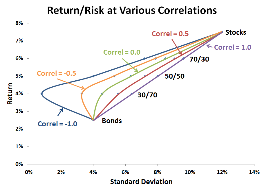
The purple line is the extreme case of perfect correlation (+1.0) between the two assets, which results in no diversification benefit and no risk reduction. The red line is a correlation of +0.5, a realistic level with a modest but important level of risk reduction. The green line is a zero correlation between the two assets, and a significant reduction in risk. With the introduction of a -0.5 correlation in the orange line we get a “bend back” extreme risk reduction such that the conservative portfolio actually has less risk than the 10-Year Treasury Bond alone. The dark blue line is the extreme case of a -1.0 correlation and a commensurately extreme level of risk reduction.
Any improvement in the return/risk tradeoff is worth pursuing and can amount to significant differences in ending wealth. For example, the 50/50 portfolio under the assumption of a -1.0 correlation has exactly the same 4% standard deviation as the 10-Year Treasury Bond, but instead of an expected return of 2.5%, the expected return on the 50/50 portfolio is 5%.
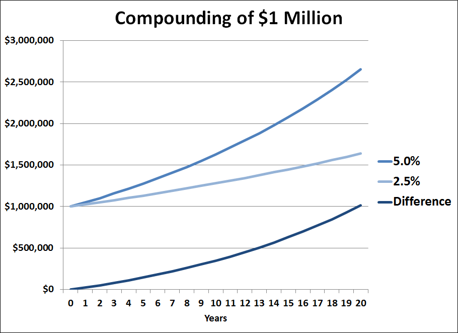
As illustrated above, a retirement nest egg of $1,000,000 will compound to $1,638,616 over 20 years at 2.5%. However, it will compound to $2,653,298 over 20 years at 5%, a difference of $1,014,681! That’s about 62% more ending retirement wealth, which could make quite a difference in lifestyle!
It pays to diversify. And the best diversification benefits are found among investments with the lowest correlation to each other.
1For the mathematically inclined, the formula for calculating portfolio return is simply the percentage weight of each asset multiplied by its expected return. The formula for calculating portfolio standard deviation (in Excel) with two assets (S and B) is as follows:
SQRT((WtB^2*SDB^2)+(WtS^2*SDS^2)+2*(WtB*SDB*WtS*SDS*CorrelSB))
Where,
WtB = % weight of asset B
SDB = standard deviation of asset B
WtS = % weight of asset S
SDS = standard deviation of asset S
CorrelSB = correlation of assets S and B